Data Preprocessing: Whitening or Sphering in Python

Outline of the post:

What is Whitening or Sphering? Why?
Steps to Whiten a dataset
Mathematical intuition
Implementation of Whitening in Python

What is Whitening or Sphering? Why?

“A whitening transformation or sphering transformation is a linear transformation that transforms a vector of random variables with a known covariance matrix into a set of new variables whose covariance is the identity matrix, meaning that they are uncorrelated and each have variance.The transformation is called “whitening” because it changes the input vector into a white noise vector.”
– Whitening Transformation, Wikipedia, 2020

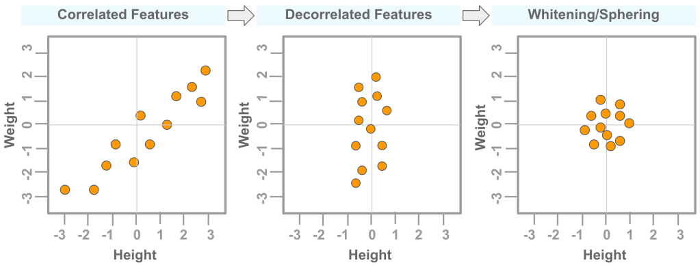
Whitening or Sphering is a data pre-processing step. It can be used to remove correlation or dependencies between features in a dataset. This may help to better train a machine learning model. Figure 1 below shows the effect of decorrelation and whitening on a data that has correlated features (‘orange’ color dots).

**Figure 1**: Example plots showing correlated features (left), decorrelated features (middle) and Whitening or Sphering (right).

Steps to Whiten a dataset

Eigenvalues and eigenvectors are first calculated from the covariance of a zero centered data set. These are then used for Whitening the data using either PCA (principal component analysis) or ZCA (zero component analysis method).

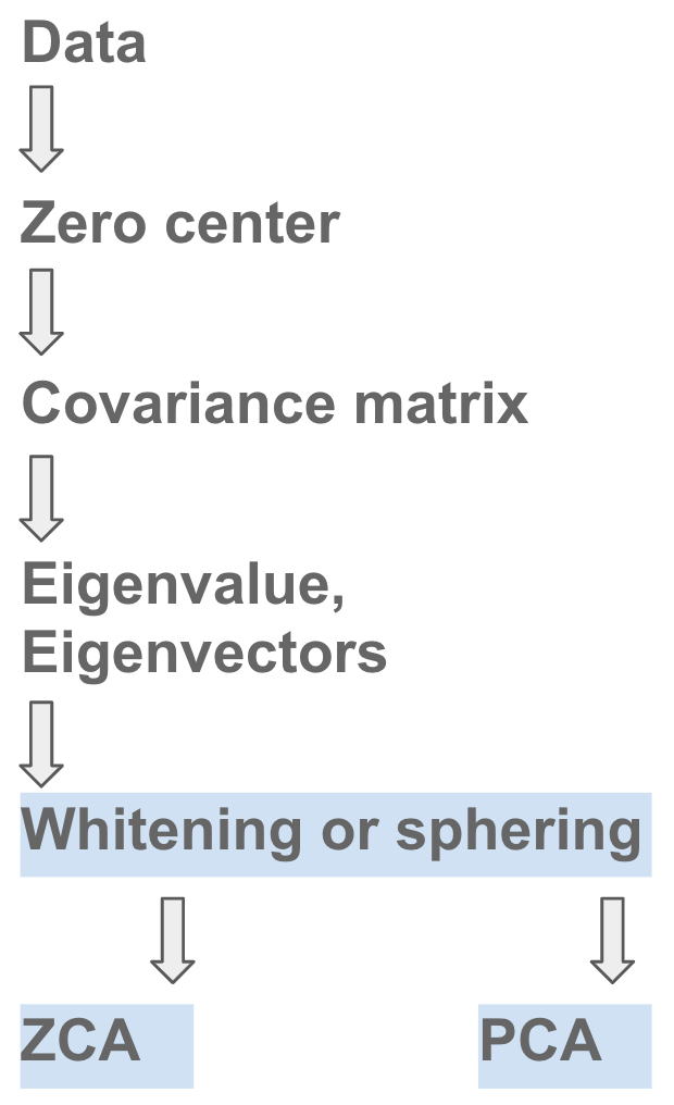
Step # 1: Find if data has one feature per row or one feature per column
Step # 2: Zero-center the dataset
Step # 3: Calculate the Covariance matrix using the zero-centered dataset
Step # 4: Calculate the Eigenvalues and Eigenvectors
Step # 5: Apply the Eigenvalues and Eigenvectors to the data for whitening transform.

Mathematical Intuition

Zero-center data:

Equation 1: Zero center using mean

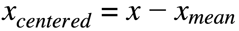
where,

x_centered: centered data for a feature
x: is individual data point for a feature
x_mean: mean value for a feature

Covariance matrix:

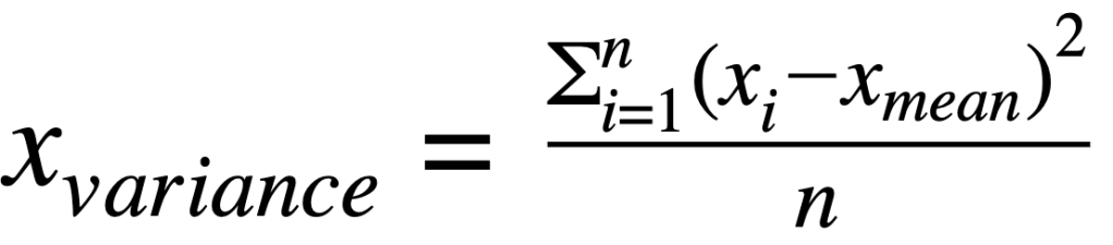
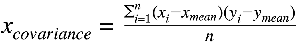
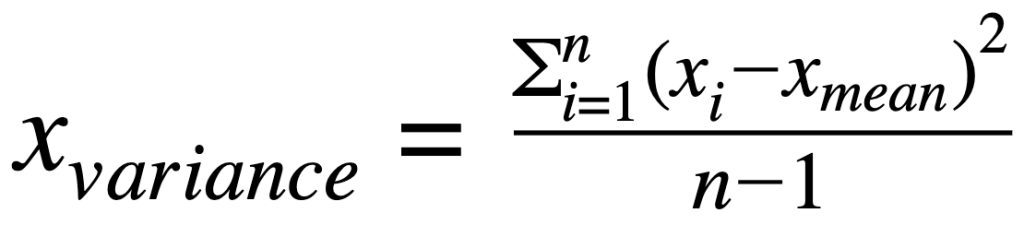
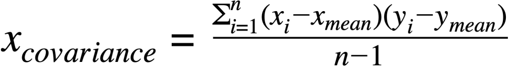
where:

x_variance: is variance for a feature
x_covariance: is covariance between features x and y
x_i and y_i: is individual data point for feature x and y
x_mean and y_mean: mean value for features x and y
∑: indicates sum of values
n: is the number of observations for a feature

Eigenvalues and Eigenvectors:

Equation 6: Substitute covariance matrix for ‘A’ and solve the simultaneous equations to calculate ‘λ’ i.e. Eigenvalues

Equation 7: Substitute the Eigenvalues ‘λ’ from above Equation#6 along with the covariance matrix ‘A’ to calculate the Eigenvectors.

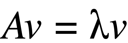
where:

A: Covariance matrix of features
λ: is the matrix for Eigenvalues
I: is identity matrix
v: is the matrix for Eigenvectors

Whitening using PCA:

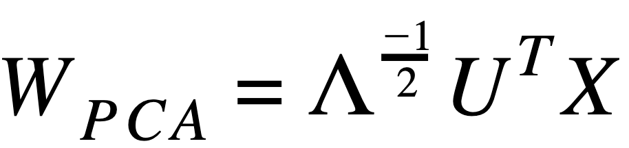
**Equation 8**: Whitening transformation using PCA

where:

X: Feature data
Λ: is the matrix for Eigenvalues (above is inverse square root)
U^T: is transpose of matrix for Eigenvectors

Whitening using ZCA:

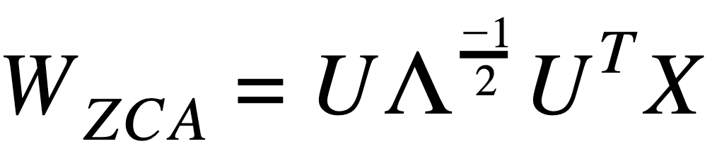
Equation 9: Whitening transformation using ZCA.

where:

X: Feature data
Λ: is the matrix for Eigenvalues (above is inverse square root)
U^T: is transpose of matrix for Eigenvectors

Implementation of Whitening in Python

Example # 1: (with 5 data points)

# Import libraries
import numpy as np
import matplotlib.pyplot as plt
from scipy import linalg

# Create data
x = np.array([[1,2,3,4,5],  # Feature-1: Height
              [11,12,13,14,15]]) # Feature-2: Weight
print('x.shape:', x.shape)

# Center data
# By subtracting mean for each feature
xc = x.T - np.mean(x.T, axis=0)
xc = xc.T
print('xc.shape:', xc.shape, '\n')

# Calculate covariance matrix
xcov = np.cov(xc, rowvar=True, bias=True)
print('Covariance matrix: \n', xcov, '\n')

# Calculate Eigenvalues and Eigenvectors
w, v = linalg.eig(xcov)
# Note: Use w.real.round(4) to (1) remove 'j' notation to real, (2) round to '4' significant digits
print("Eigenvalues:\n", w.real.round(4), '\n')
print("Eigenvectors:\n", v, '\n')

# Calculate inverse square root of Eigenvalues
# Optional: Add '.1e5' to avoid division errors if needed
# Create a diagonal matrix
diagw = np.diag(1/(w**0.5)) # or np.diag(1/((w+.1e-5)**0.5))
diagw = diagw.real.round(4) #convert to real and round off
print("Diagonal matrix for inverse square root of Eigenvalues:\n", diagw, '\n')

# Calculate Rotation (optional)
# Note: To see how data can be rotated
xrot = np.dot(v, xc)

# Whitening transform using PCA (Principal Component Analysis)
wpca = np.dot(np.dot(diagw, v.T), xc)

# Whitening transform using ZCA (Zero Component Analysis)
wzca = np.dot(np.dot(np.dot(v, diagw), v.T), xc)

# Plot zero-centered, rotated and whitened data
plt.scatter(xc[0,:], xc[1,:], s=150, label='centered', alpha=0.5)
plt.scatter(xrot[0,:], xrot[1,:], s=150, label='rotated')
plt.scatter(wpca[0,:], wpca[1,:], s=150, marker='+', label='wpca')
plt.scatter(wzca[0,:], wzca[1,:], s=150, marker='x', label='wzca')
plt.xlabel('Height', fontsize=16)
plt.ylabel('Weight', fontsize=16)
plt.rc('xtick',labelsize=16)
plt.rc('ytick',labelsize=16)
plt.legend()
plt.tight_layout()
plt.savefig('whiten_1.png', dpi=300)

x.shape: (2, 5)
xc.shape: (2, 5) 

Covariance matrix: 
 [[2. 2.]
 [2. 2.]] 

Eigenvalues:
 [4. 0.] 

Eigenvectors:
 [[ 0.70710678 -0.70710678]
 [ 0.70710678  0.70710678]] 

Diagonal matrix for inverse square root of Eigenvalues:
 [[5.00000000e-01 0.00000000e+00]
 [0.00000000e+00 4.74531328e+07]]

**Figure 2**: The plot shows the original centered data, rotated data as well as the whitening transformed data using PCA and ZCA

Example # 2: (1000 data points)

# Import libraries
import numpy as np
import matplotlib.pyplot as plt
from scipy import linalg

# Create data
np.random.seed(1)
mu = [0,0]
sigma = [[6,5], [5,6]]
n = 1000
x = np.random.multivariate_normal(mu, sigma, size=n)
print('x.shape:', x.shape, '\n')

# Zero center data
xc = x - np.mean(x, axis=0)
print(xc.shape)
xc = xc.T
print('xc.shape:', xc.shape, '\n')

# Calculate Covariance matrix
# Note: 'rowvar=True' because each row is considered as a feature
# Note: 'bias=True' to divide the sum of squared variances by 'n' instead of 'n-1'
xcov = np.cov(xc, rowvar=True, bias=True)
print

# Calculate Eigenvalues and Eigenvectors
w, v = linalg.eig(xcov) # .eigh()
# Note: Use w.real.round(4) to (1) remove 'j' notation to real, (2) round to '4' significant digits
print("Eigenvalues:\n", w.real.round(4), '\n')
print("Eigenvectors:\n", v, '\n')

# Calculate inverse square root of Eigenvalues
# Optional: Add '.1e5' to avoid division errors if needed
# Create a diagonal matrix
diagw = np.diag(1/(w**0.5)) # or np.diag(1/((w+.1e-5)**0.5))
diagw = diagw.real.round(4) #convert to real and round off
print("Diagonal matrix for inverse square root of Eigenvalues:\n", diagw, '\n')

# Calculate Rotation (optional)
# Note: To see how data can be rotated
xrot = np.dot(v, xc)

# Whitening transform using PCA (Principal Component Analysis)
wpca = np.dot(np.dot(diagw, v.T), xc)

# Whitening transform using ZCA (Zero Component Analysis)
wzca = np.dot(np.dot(np.dot(v, diagw), v.T), xc)


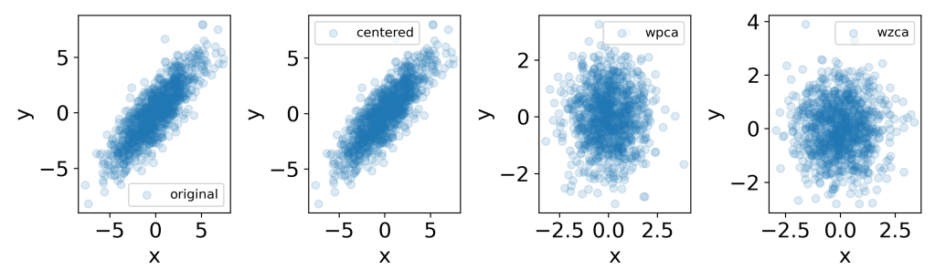
fig = plt.figure(figsize=(10,3))

plt.subplot(1,4,1)
plt.scatter(x[:,0], x[:,1], label='original', alpha=0.15)
plt.xlabel('x', fontsize=16)
plt.ylabel('y', fontsize=16)
plt.legend()

plt.subplot(1,4,2)
plt.scatter(xc[0,:], xc[1,:], label='centered', alpha=0.15)
plt.xlabel('x', fontsize=16)
plt.ylabel('y', fontsize=16)
plt.legend()

plt.subplot(1,4,3)
plt.scatter(wpca[0,:], wpca[1,:], label='wpca', alpha=0.15)
plt.xlabel('x', fontsize=16)
plt.ylabel('y', fontsize=16)
plt.legend()

plt.subplot(1,4,4)
plt.scatter(wzca[0,:], wzca[1,:], label='wzca', alpha=0.15)
plt.xlabel('x', fontsize=16)
plt.ylabel('y', fontsize=16)
plt.legend()

plt.tight_layout()
plt.savefig('whiten_2.png', dpi=300)

x.shape: (1000, 2) 

(1000, 2)
xc.shape: (2, 1000) 

Eigenvalues:
 [ 1.005  11.1862] 

Eigenvectors:
 [[-0.71582163 -0.69828318]
 [ 0.69828318 -0.71582163]] 

Diagonal matrix for inverse square root of Eigenvalues:
 [[0.9975 0.    ]
 [0.     0.299 ]]

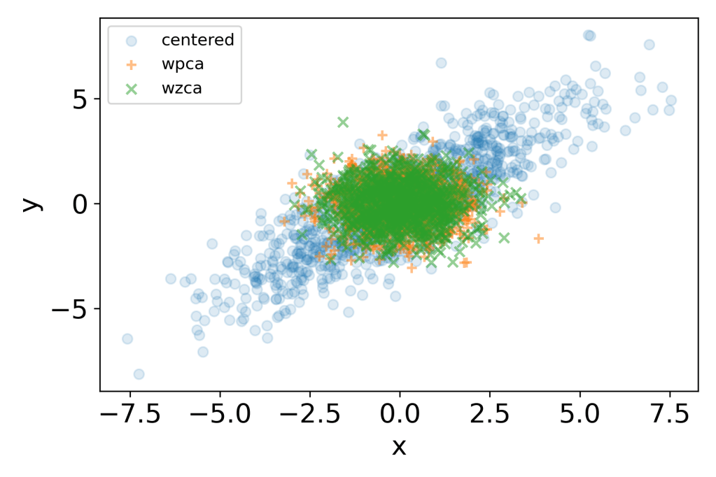
# Overlay plot
plt.scatter(xc[0,:], xc[1,:], label='centered', alpha=0.15)
plt.scatter(wpca[0,:], wpca[1,:], marker='+',label='wpca', alpha=0.5)
plt.scatter(wzca[0,:], wzca[1,:], marker='x', label='wzca', alpha=0.5)
plt.xlabel('x', fontsize=16)
plt.ylabel('y', fontsize=16)
plt.legend()

plt.tight_layout()
plt.savefig('whiten_3.png', dpi=300)

Check out the explanation on YouTube video!

Share this:

Related

Leave a comment Cancel reply