Outline of the post:
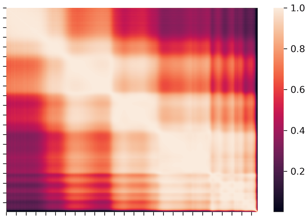
This post shows an implementation of the PLS-W2A algorithm from in Python using the source code from Scikit-learn docs. Partial Least Squares method can be used in datasets that have collinear features such as shown in figure above. [Check out videos: 1, 2, and project]
References:
(1) Jacob A. Wegelin. A survey of Partial Least Squares (PLS) methods, with emphasis on the two-block case. Technical Report No. 371. Department of Statistics, University of Washington, Seattle, USA, March 2000.[PDF]
(2) Cross-decomposition, Scikit-learn [docs][Source code]
.
PLS-W2A algorithm[1]
The steps for the PLS-W2A (Wold’s Two-Block, Mode A PLS) algorithm as below:
Step # 0:
Standardize both the feature matrix X and the target matrix Y

Step # 1:
Begin iteration

Step # 2:
Feature matrix (n x d) : X
Target matrix (n x t): Y

Step # 3:
Calculate the cross-covariance C matrix between X and Y to find the singular vectors u and v i.e. weights

Step # 4:
Project on singular vectors to get the scores.

Step # 5:
Regress on X and Y on scores to get the loadings

Step # 6:
Deflate

Step # 7:
Check condition

Step # 8:

Step # 9:

Code
The code below implements the above algorithm and is based on the source code from Scikit-learn.[Source code]
######################
# Import libraries
######################
import numpy as np
import matplotlib.pyplot as plt
from sklearn.cross_decomposition import PLSCanonical
from scipy.linalg import svd, pinv2

######################
# Functions
######################
def _svd_flip_1d(u, v):
    biggest_abs_val_idx = np.argmax(np.abs(u))
    sign = np.sign(u[biggest_abs_val_idx])
    u *= sign
    v *= sign


def _center_scale_xy(X, Y, scale=True):
    # center
    x_mean = X.mean(axis=0)
    X -= x_mean
    y_mean = Y.mean(axis=0)
    Y -= y_mean
    # scale
    if scale:
        x_std = X.std(axis=0, ddof=1)
        x_std[x_std == 0.0] = 1.0
        X /= x_std
        y_std = Y.std(axis=0, ddof=1)
        y_std[y_std == 0.0] = 1.0
        Y /= y_std
    else:
        x_std = np.ones(X.shape[1])
        y_std = np.ones(Y.shape[1])
    return X, Y, x_mean, y_mean, x_std, y_std


###########
# Data
###########

X = np.array([
    [2.88,-0.35,-0.07,0.27],
    [-1.03, -0.13, -1.01, -0.45],
    [0.91,-0.97,1.08,-1.48],
    [0.79,-0.69,-0.32,1.42],
    [0.62,-1.11,0.65,0.13]
])

Y = np.array([
    [2.742, 2.966, 0.195, 3.061, 2.119],
    [-2.385, -6.058, -1.357, -1.829,-2.618],
    [-0.421,-3.631, 0.252, -0.703,-0.799],
    [0.989,4.085,0.279,1.698,-0.149],
    [0.251,0.84,0.865,0.545,-0.922]
])


plt.scatter(X[:,0], X[:,1])
plt.show()
plt.scatter(Y[:,0], Y[:,1])
plt.show()

X_orig = X.copy()

print("X:\n", X, "\n Y:\n", Y, '\n\n')

######################
# PLS-W2A algorithm
######################
n_components=1
n = X.shape[0]
p = X.shape[1]
q = Y.shape[1]

x_weights_ = np.zeros((p, n_components))  # U
y_weights_ = np.zeros((q, n_components))  # V
_x_scores = np.zeros((n, n_components))  # Xi
_y_scores = np.zeros((n, n_components))  # Omega
x_loadings_ = np.zeros((p, n_components))  # Gamma
y_loadings_ = np.zeros((q, n_components))  # Delta
n_iter_=[]

Xk, Yk, _x_mean, _y_mean, _x_std, _y_std = _center_scale_xy(X.copy(), Y.copy())

Y_eps=np.finfo(Yk.dtype).eps
max_iter=500
algorithm = 'svd'
deflation_mode = 'canonical'
mode = 'A'
tol=1e-6

if deflation_mode == 'canonical':
    rank_upper_bound = p
else:
    rank_upper_bound = min(n, p, q)

_norm_y_weights = (deflation_mode == 'canonical')  # 1.1
norm_y_weights = _norm_y_weights

for k in range(n_components):
    print('-'*50, k, '-'*50)
    ################################
    # Weights: uk, vk
    ################################
    C = np.dot(Xk.T, Yk)
    U, S, Vt = svd(C, full_matrices=False)
    # U --> Left singular values
    # S --> Singular values (diagonal)
    # V --> Right singular vectors
    # C = np.dot(U, np.dot(S*np.eye(4,4), Vt))
    print('\n')
    print('C:\n', C.round(2), '\n') # covariance
    print('U:\n', U.round(2), '\n') #  rotation
    print('S:\n', S.round(2), '\n') # stretches ... stores equivalent of lambda
    print('Vt:\n', Vt.round(2), '\n\n') #  rotation


    x_weights, y_weights =  U[:, 0], Vt[0, :]
    print("np.dot(U[:, 0].T, U[:, 0]):", np.dot(U[:, 0].T, U[:, 0]).round(2), '\n')
    print("np.dot(Vt[0, :].T, Vt[0, :]):", np.dot(Vt[0, :].T, Vt[0, :]).round(2), '\n\n')

    _svd_flip_1d(x_weights, y_weights)

    ################################
    # Scores: eta_k, w_k
    ################################
    # compute scores, i.e. the projections of X and Y
    x_scores = np.dot(Xk, x_weights)   # eta_k
    if norm_y_weights:
        y_ss = 1
    else:
        y_ss = np.dot(y_weights, y_weights)
    y_scores = np.dot(Yk, y_weights) / y_ss  #w_k


    ################################
    # Loadings: gamma_k, delta_k
    ################################
    # Deflation: subtract rank-one approx to obtain Xk+1 and Yk+1
    print('-- matrix ---')
    print('Xk:\n', Xk, '\n')

    x_loadings = np.dot(x_scores, Xk) / np.dot(x_scores, x_scores)  #
    Xk -= np.outer(x_scores, x_loadings)


    print('np.outer(x_scores, x_loadings):\n', np.outer(x_scores, x_loadings), '\n')
    print('Xk (after substract):\n', Xk )
    print('------','\n\n')


    if deflation_mode == "canonical":
        # regress Yk on y_score
        y_loadings = np.dot(y_scores, Yk) / np.dot(y_scores, y_scores)
        Yk -= np.outer(y_scores, y_loadings)  # np.outer() is same as .T i.e. transpose
    if deflation_mode == "regression":
        # regress Yk on x_score
        y_loadings = np.dot(x_scores, Yk) / np.dot(x_scores, x_scores)
        Yk -= np.outer(x_scores, y_loadings)

    x_weights_[:, k] = x_weights # uk
    y_weights_[:, k] = y_weights # vk
    _x_scores[:, k] = x_scores   # epsilon_k
    _y_scores[:, k] = y_scores   # w_k
    x_loadings_[:, k] = x_loadings # gamma_k
    y_loadings_[:, k] = y_loadings # delta_k

    print("x_weights_:\n", x_weights_, '\n')
    print("y_weights_:\n", y_weights_, '\n')
    print("_x_scores:\n", _x_scores, '\n' )
    print("_y_scores:\n", _y_scores, '\n' )
    print("x_loadings_:\n", x_loadings_, '\n' )
    print("y_loadings_:\n", y_loadings_, '\n' )

    # Compute transformation matrices (rotations_). See User Guide.
    x_rotations_ = np.dot(
        x_weights_,
        pinv2(np.dot(x_loadings_.T, x_weights_),check_finite=False))

    y_rotations_ = np.dot(
        y_weights_, pinv2(np.dot(y_loadings_.T, y_weights_),check_finite=False))

    coef_ = np.dot(x_rotations_, y_loadings_.T)
    coef_ = coef_ * _y_std

    print('\ncoef_:\n', coef_,'\n')
    print('Xk:\n', Xk, '\n')
    print("Yk:\n", Yk, '\n')


########################################################
# Compare output with .PLSCanonical() from Scikit-learn
########################################################
# PLSCanonical
print('='*25)
plsca = PLSCanonical(n_components=2, algorithm=algorithm, scale=True)
plsca.fit(X,Y)

print("PLSCanonical: x_weights:\n", plsca.x_weights_, '\n')
print("Calculated: x_weights_:\n", x_weights_, '\n')
Output:
X:
 [[ 2.88 -0.35 -0.07  0.27]
 [-1.03 -0.13 -1.01 -0.45]
 [ 0.91 -0.97  1.08 -1.48]
 [ 0.79 -0.69 -0.32  1.42]
 [ 0.62 -1.11  0.65  0.13]]
 Y:
 [[ 2.742  2.966  0.195  3.061  2.119]
 [-2.385 -6.058 -1.357 -1.829 -2.618]
 [-0.421 -3.631  0.252 -0.703 -0.799]
 [ 0.989  4.085  0.279  1.698 -0.149]
 [ 0.251  0.84   0.865  0.545 -0.922]]


-------------------------------------------------- 0 --------------------------------------------------


C:
 [[ 3.8   2.77  2.38  3.52  3.93]
 [-0.57 -0.92 -3.33 -0.16 -0.06]
 [ 0.99  0.38  3.06  0.32  0.88]
 [ 1.96  3.21  0.91  2.56  1.4 ]]

U:
 [[ 0.8   0.22 -0.5   0.26]
 [-0.24  0.7  -0.36 -0.56]
 [ 0.27 -0.6  -0.21 -0.72]
 [ 0.49  0.31  0.76 -0.3 ]]

S:
 [9.25 3.78 1.74 0.01]

Vt:
 [[ 0.47  0.44  0.43  0.45  0.44]
 [ 0.12  0.2  -0.89  0.34  0.19]
 [-0.24  0.74  0.03  0.1  -0.61]
 [ 0.08 -0.46  0.09  0.74 -0.47]]


np.dot(U[:, 0].T, U[:, 0]): 1.0

np.dot(Vt[0, :].T, Vt[0, :]): 1.0


-- matrix ---
Xk:
 [[ 1.47330421  0.72975638 -0.16570217  0.27540185]
 [-1.34224782  1.26491106 -1.31099659 -0.40367121]
 [ 0.05472684 -0.77840681  1.23545589 -1.37512294]
 [-0.03168396 -0.09730085 -0.47030175  1.36003243]
 [-0.15409927 -1.11895979  0.71154462  0.14335987]]

np.outer(x_scores, x_loadings):
 [[ 0.8379257  -0.41891981  0.45663276  0.41189286]
 [-1.47398529  0.73691695 -0.80325735 -0.72455592]
 [-0.0854582   0.04272471 -0.04657097 -0.04200805]
 [ 0.41132775 -0.20564275  0.22415559  0.20219331]
 [ 0.31019004 -0.15507909  0.16903997  0.15247779]]

Xk (after substract):
 [[ 0.63537851  1.1486762  -0.62233493 -0.13649101]
 [ 0.13173747  0.52799412 -0.50773924  0.32088471]
 [ 0.14018504 -0.82113152  1.28202686 -1.3331149 ]
 [-0.44301172  0.1083419  -0.69445734  1.15783913]
 [-0.4642893  -0.9638807   0.54250465 -0.00911793]]
------


x_weights_:
 [[ 0.79639603  0.        ]
 [-0.23755967  0.        ]
 [ 0.26769172  0.        ]
 [ 0.48750375  0.        ]]

y_weights_:
 [[0.4735017  0.        ]
 [0.44247997 0.        ]
 [0.42756377 0.        ]
 [0.45154019 0.        ]
 [0.4396684  0.        ]]

_x_scores:
 [[ 1.08987528  0.        ]
 [-1.91718685  0.        ]
 [-0.11115398  0.        ]
 [ 0.53500681  0.        ]
 [ 0.40345875  0.        ]]

_y_scores:
 [[ 2.29929773  0.        ]
 [-3.07210752  0.        ]
 [-0.77102556  0.        ]
 [ 1.11359293  0.        ]
 [ 0.43024241  0.        ]]

x_loadings_:
 [[ 0.76882714  0.        ]
 [-0.38437409  0.        ]
 [ 0.41897708  0.        ]
 [ 0.37792661  0.        ]]

y_loadings_:
 [[0.48157766 0.        ]
 [0.45578485 0.        ]
 [0.3672144  0.        ]
 [0.47494814 0.        ]
 [0.45222887 0.        ]]


coef_:
 [[ 0.72130924  1.57623961  0.24284168  0.72886412  0.61680754]
 [-0.21516177 -0.47018185 -0.07243807 -0.21741535 -0.18398961]
 [ 0.24245288  0.52981969  0.08162611  0.2449923   0.20732684]
 [ 0.44154032  0.96487513  0.14865246  0.44616495  0.37757093]]

Xk:
 [[ 0.63537851  1.1486762  -0.62233493 -0.13649101]
 [ 0.13173747  0.52799412 -0.50773924  0.32088471]
 [ 0.14018504 -0.82113152  1.28202686 -1.3331149 ]
 [-0.44301172  0.1083419  -0.69445734  1.15783913]
 [-0.4642893  -0.9638807   0.54250465 -0.00911793]]

Yk:
 [[ 0.22559743 -0.28214736 -0.66586174  0.20876244  0.47412439]
 [ 0.08627471  0.08796074 -0.56243867  0.22221725  0.13729959]
 [ 0.02240131 -0.40193446  0.53024886 -0.28633537  0.15879608]
 [-0.13547932  0.51596848 -0.12929478  0.06457668 -0.3139485 ]
 [-0.19879414  0.0801526   0.82734634 -0.209221   -0.45627155]]

-------------------------------------------------- 1 --------------------------------------------------


C:
 [[ 0.31 -0.49 -0.75  0.19  0.69]
 [ 0.46  0.03 -2.31  0.8   0.89]
 [-0.17 -0.7   1.92 -0.77 -0.19]
 [-0.19  1.2  -0.95  0.5  -0.59]]

U:
 [[-0.22  0.5   0.26 -0.8 ]
 [-0.71  0.36 -0.56  0.24]
 [ 0.6   0.22 -0.72 -0.27]
 [-0.31 -0.76 -0.3  -0.49]]

S:
 [3.63 1.74 0.01 0.  ]

Vt:
 [[-0.12 -0.19  0.89 -0.34 -0.2 ]
 [ 0.24 -0.74 -0.03 -0.1   0.61]
 [ 0.08 -0.46  0.09  0.74 -0.47]
 [-0.95 -0.26 -0.18 -0.01  0.05]]


np.dot(U[:, 0].T, U[:, 0]): 1.0

np.dot(Vt[0, :].T, Vt[0, :]): 1.0


-- matrix ---
Xk:
 [[ 0.63537851  1.1486762  -0.62233493 -0.13649101]
 [ 0.13173747  0.52799412 -0.50773924  0.32088471]
 [ 0.14018504 -0.82113152  1.28202686 -1.3331149 ]
 [-0.44301172  0.1083419  -0.69445734  1.15783913]
 [-0.4642893  -0.9638807   0.54250465 -0.00911793]]

np.outer(x_scores, x_loadings):
 [[ 0.1580263   0.81373251 -0.82624044  0.59206977]
 [ 0.09888346  0.50918542 -0.51701214  0.37048206]
 [-0.21170698 -1.09015304  1.10690984 -0.79319266]
 [ 0.09163572  0.47186429 -0.47911734  0.34332729]
 [-0.13683851 -0.70462918  0.71546008 -0.51268645]]

Xk (after substract):
 [[ 0.47735221  0.33494369  0.20390551 -0.72856078]
 [ 0.03285401  0.0188087   0.0092729  -0.04959734]
 [ 0.35189201  0.26902152  0.17511702 -0.53992224]
 [-0.53464744 -0.36352239 -0.21533999  0.81451183]
 [-0.3274508  -0.25925152 -0.17295543  0.50356853]]
------


x_weights_:
 [[ 0.79639603  0.22436662]
 [-0.23755967  0.70787937]
 [ 0.26769172 -0.59593871]
 [ 0.48750375  0.30565253]]

y_weights_:
 [[ 0.4735017   0.12150951]
 [ 0.44247997  0.19162239]
 [ 0.42756377 -0.8921763 ]
 [ 0.45154019  0.3364049 ]
 [ 0.4396684   0.19841748]]

_x_scores:
 [[ 1.08987528  1.28483657]
 [-1.91718685  0.80397433]
 [-0.11115398 -1.72128859]
 [ 0.53500681  0.74504642]
 [ 0.40345875 -1.11256872]]

_y_scores:
 [[ 2.29929773  0.73171581]
 [-3.07210752  0.63113051]
 [-0.77102556 -0.61218984]
 [ 1.11359293  0.15719387]
 [ 0.43024241 -0.90785036]]

x_loadings_:
 [[ 0.76882714  0.12299331]
 [-0.38437409  0.63333542]
 [ 0.41897708 -0.64307046]
 [ 0.37792661  0.46081329]]

y_loadings_:
 [[ 0.48157766  0.16917896]
 [ 0.45578485  0.04795733]
 [ 0.3672144  -0.89840858]
 [ 0.47494814  0.30980952]
 [ 0.45222887  0.32503774]]


coef_:
 [[ 0.85193267  1.66173386 -0.06342306  0.97394799  0.84533836]
 [-0.00759823 -0.33432957 -0.55909958  0.17202839  0.17915096]
 [ 0.07274775  0.41874609  0.47952333 -0.07341912 -0.08957895]
 [ 0.57505242  1.05226004 -0.16438514  0.6966687   0.61115557]]

Xk:
 [[ 0.47735221  0.33494369  0.20390551 -0.72856078]
 [ 0.03285401  0.0188087   0.0092729  -0.04959734]
 [ 0.35189201  0.26902152  0.17511702 -0.53992224]
 [-0.53464744 -0.36352239 -0.21533999  0.81451183]
 [-0.3274508  -0.25925152 -0.17295543  0.50356853]]

Yk:
 [[ 0.10180651 -0.3172385  -0.00848198 -0.01793009  0.23628913]
 [-0.02049929  0.05769341  0.00457439  0.02668701 -0.06784165]
 [ 0.12597095 -0.37257547 -0.01974774 -0.09667313  0.35778088]
 [-0.16207321  0.50842988  0.01192954  0.01587653 -0.36504244]
 [-0.04520496  0.12369068  0.01172579  0.07203968 -0.16118592]]

=========================
PLSCanonical: x_weights:
 [[ 0.79639603  0.22436662]
 [-0.23755967  0.70787937]
 [ 0.26769172 -0.59593871]
 [ 0.48750375  0.30565253]]

Calculated: x_weights_:
 [[ 0.79639603  0.22436662]
 [-0.23755967  0.70787937]
 [ 0.26769172 -0.59593871]
 [ 0.48750375  0.30565253]]
Check out the related YouTube videos!
